How I drew
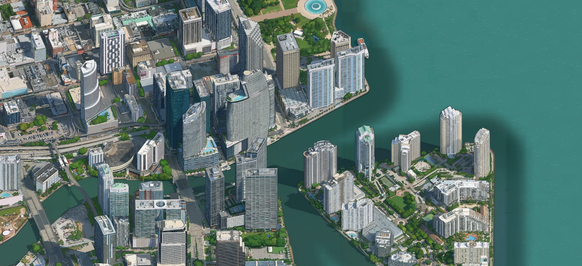
Miami in pixels

One angle for the whole city

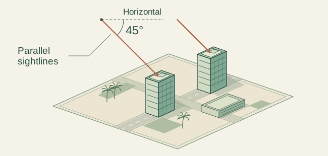
I used Cesium to look at Google’s 3D model of Brickell from 45° above the ground, facing 15° east of north. From there I could see the shape of a roof and the windows down its side in the same picture.

I used an orthographic camera. Its sightlines run parallel, so a tower at the far side of the picture stays the same size as an identical tower up close. I slid the camera across Brickell at that fixed angle and fitted 72 frames together. Each pixel represented 25 centimetres along the image.

The balcony test

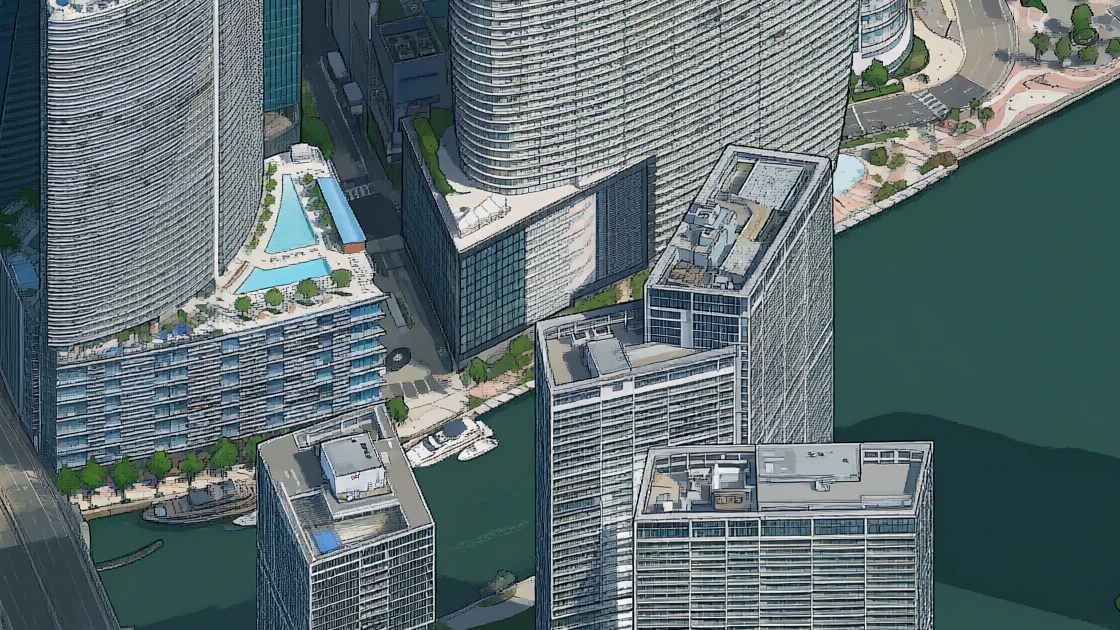
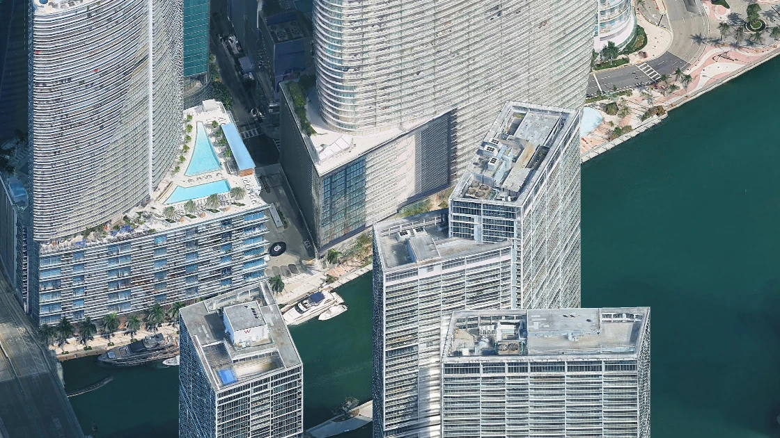
Icon Brickell has long bands of balconies that curve around the towers. I put one of those curves right where four drawing windows met. If each window drew its own idea of the building, I’d be able to see the break in a single balcony line.

Pixel artwork

3D capture

Imagery © Google · Vexcel Imaging US, Inc.

On my M1 Max, I tried Qwen-Image-2.1-Turbo with Boris Starkov’s Tiny London style adapter, a set of weights that gives the model its pixel-art look. Qwen drew in windows 1,024 pixels wide. Each window shared 256 pixels with its neighbor, and on each drawing pass their predictions were averaged in that overlap. On the next pass the windows shifted, putting the old joins closer to the middle of the drawing.

When I extended the map south, I gave the model a strip of the finished drawing to work from and kept those pixels fixed. One join near Flatiron still broke a curve in the elevated tracks. Redrawing a strip just 64 pixels high let the tracks meet again.

Renting GPUs to draw the city

One 2,560-pixel-square Brickell patch took 27 minutes and 45 seconds on my M1 Max. To see what renting a GPU would buy me, I sent the same crop, model and drawing instructions to an NVIDIA L40S on Modal. The first render took four minutes. A second run on the same worker took two.

My Mac kept the job list. Downtown and Bayside could draw at the same time because each had a finished edge from Brickell to work from. Port Boulevard needed an edge from both, so it waited. As each drawing came back, the Mac checked that the shared pixels still matched and saved the result. If a run stopped, the queue could pick up at the first unfinished patch.

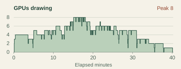
For Overtown, Wynwood and Edgewater, I set a ceiling of ten rented GPUs. At the busiest point, eight were drawing at once. They handled 71 patches, and the Mac drew two patches that were entirely open water. That 73-patch batch finished in 40 minutes and 15 seconds. Modal metered $7.80 before credits for those three neighborhoods.

Where the drawing meets the bay

Just east of a Brickell marina, two patches of water met in a ruler-straight line. There was a real diagonal shadow in the original capture. I used it as a reference, matching the color across the join while keeping the shadow, boats and docks in place.

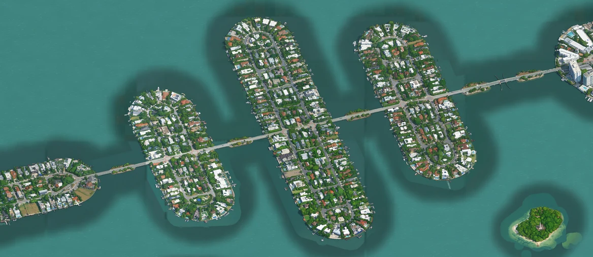
I kept the model’s painted shoreline wherever I could match it to its exact place on the map. For banks with gaps, I took four small samples of model-painted water from Edgewater, checked each one for bits of boats or buildings, and blended its opposite edges so it could repeat. Out in the bay, I placed ripples using map coordinates. Two adjoining tiles could draw opposite ends of the same ripple.

To join those textures, I made a mask that records distance from the bank. In Edgewater the shoreline has full weight through the first 32 metres in the map’s projection. It fades gradually until the offshore pattern takes over at 88 metres.

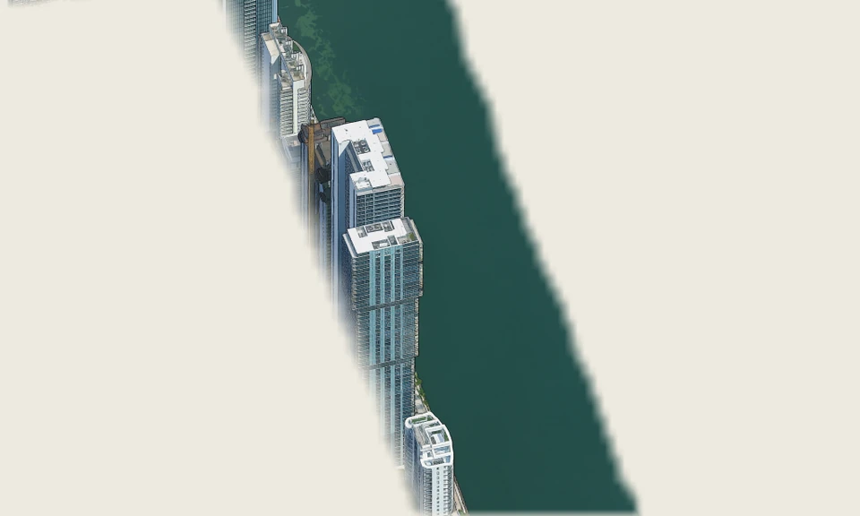Painted bank · Only the shoreline artwork is visible. The pale background marks transparent pixels.

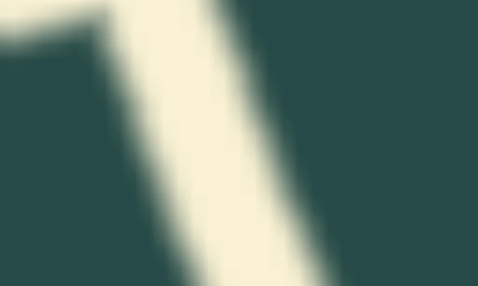Distance mask · The lightest band keeps the painted bank at full strength. Dark teal gives it zero weight.

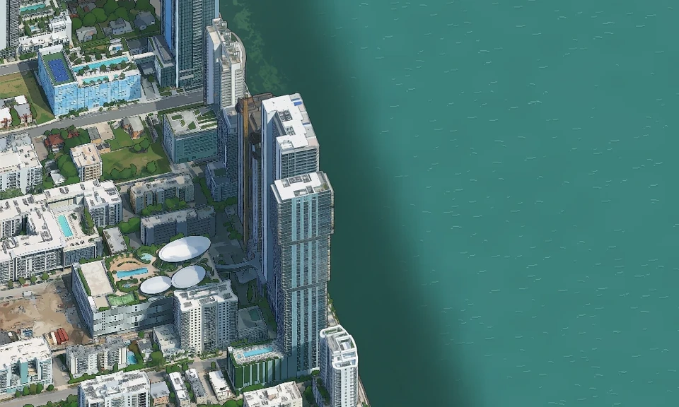Finished map · Follow the dark water beside the towers as it fades into the bay.

Drawing those layers on a phone during a pan used to make the map hitch. I moved that work into a build step. Before publishing, I ran Chrome without a visible window and used its 2D canvas to draw the city, water, foreground objects and shadows together. It wrote the result to WebP images. When you drag past Edgewater now, the painted bank and the ripples arrive in the same image as the towers.

From Biscayne Bay to one rooftop

The map eventually stretched from Aventura to Florida City. The central artwork has a quarter metre per pixel, and the wider region uses half a metre. Loading the whole picture just to look at one roof would make for a long wait.

I built a tile pyramid. Each tile is a 512-by-512-pixel image. At Bayfront Park, one tile at a metre per pixel covers the same patch of city as four tiles at half a metre per pixel. Go one level finer and it takes sixteen tiles to cover the park. The ground stays put while more pixels become available to draw the boats in the marina.

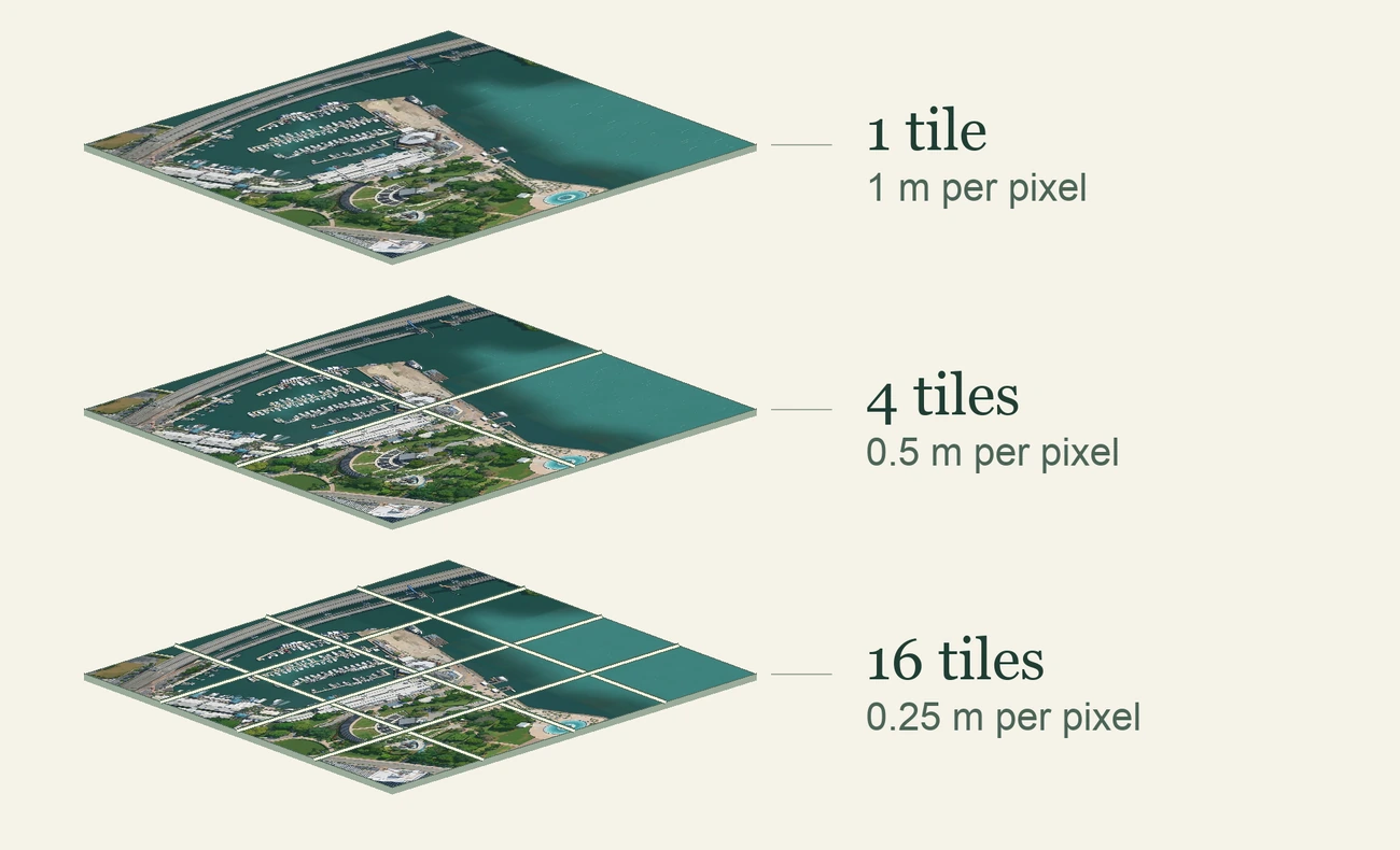
The build drew each level at its own scale. It recorded which squares had artwork and which were empty, producing 66,675 WebP tiles across ten levels. I stored neighboring tiles together in groups of up to sixteen. When the browser asks for one, the server reads just that tile’s bytes from the group.

Biscayne Bay

Downtown waterfront

Kaseya Center

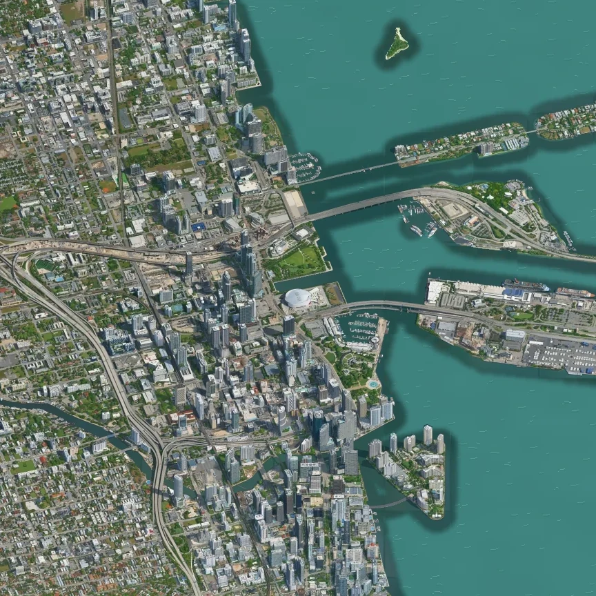
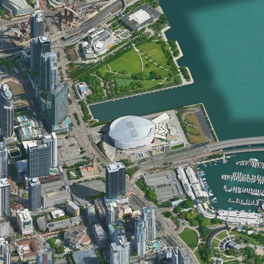
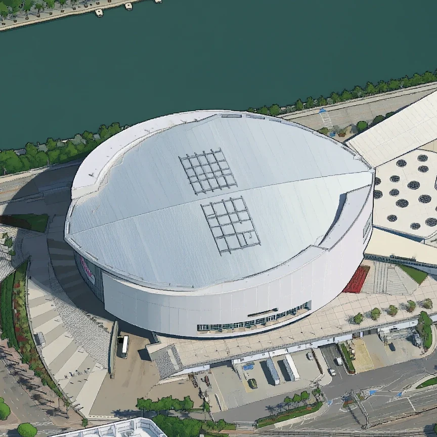
When you pinch toward Kaseya Center, the browser picks a level for the screen and gives nearby tiles priority, with up to six downloads running at once. While a sharper tile is on its way, it can enlarge the matching corner of a coarser tile already in memory. Each piece of the roof comes into focus as it arrives. Zoom back out and the browser can keep the fine pieces visible while it fetches the wider view.

What the whole map took

From the first Brickell capture on the night of November 7 to the last web tile on the morning of November 12, the map took about four days and nine hours. That includes testing on my Mac, checking the artwork and baking the tiles. Within that stretch, about 30 hours passed between my first Modal tests and the last GPU render, with several GPUs often drawing at once.

Modal recorded $228.17 in compute for the project, including the $7.80 neighborhood batch. A $30 credit brought my Modal spend to $198.17.

Credits & further reading

Built with Qwen, using the Qwen team’s image model and Boris Starkov’s Tiny London adapter. Boris also published the shared-window technique behind the Brickell test.

Isometric Los Angeles sparked the idea for Miami. I planned the work with help from Justin Chavez on San Francisco and Yadong Xie on Singapore.